


How to Hide Excel Errors with the IF and ISERROR Functions

Microsoft Excel is a powerful and versatile spreadsheet application that is great for tracking and managing everything from enterprise inventory, to small business budgets, to personal fitness. One of the benefits of Excel is that you can set up formulas ahead of time which will automatically update as you enter new data. Some formulas, unfortunately, are mathematically impossible without the requisite data, resulting in errors in your table such as #DIV/0!, #VALUE!, #REF!, and #NAME?. While not necessarily harmful, these errors will be displayed in your spreadsheet until corrected or until the required data is entered, which can make the overall table less attractive and more difficult to understand. Thankfully, at least in the case of missing data, you can hide Excel errors with some help from the IF and ISERROR functions. Here’s how to do it.
We’re using a small weight loss tracking spreadsheet as an example of the kind of table that would produce a calculation error (weight lost percentage calculation) while waiting for new data (subsequent weigh-ins).
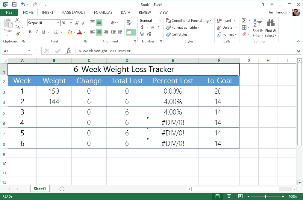
Our example spreadsheet waits for input in the Weight column and then automatically updates all other columns based upon the new data. The problem is that the Percent Lost column relies on a value, Change, that hasn’t been updated for the weeks in which weight has not yet been entered, resulting in a #DIV/0! error, which indicates that the formula is attempting to divide by zero. We can solve this error three ways:
- We can remove the formula from the weeks in which no weight has been entered, and then manually add it back in each week. This would work in our example because the spreadsheet is relatively small, but wouldn’t be ideal in larger and more complicated spreadsheets.
- We can calculate percent lost using another formula that doesn’t divide by zero. Again, this is possible in our example, but might not always be depending on the spreadsheet and data set.
- We can use the ISERROR function, which when coupled with an IF statement lets us define an alternate value or calculation if the initial result returns an error. This is the solution we’ll show you today.
The ISERROR Function
By itself, ISERROR tests the designated cell or formula and returns “true” if the result of the calculation or the value of the cell is an error, and “false” if it is not. You can use ISERROR simply by entering the calculation or cell in parentheses following the function. For example:
ISERROR((B5-B4)/C5)
If the calculation of (B5-B4)/C5 returns an error, then ISERROR will return “true” when paired with a conditional formula. While this can be utilized in many different ways, its arguably most useful role is when paired with the IF function.
The IF Function
The IF function is used by placing three tests or values in parentheses separated by commas: IF(value to be tested,value if true,value if false). For example:
IF(B5>100,0,B5)
In the example above, if the value in the cell B5 is greater than 100 (which means the test is true), then a zero will be shown as the cell value. But if B5 is less than or equal to 100 (which means the test is false), the actual value of B5 will be shown.
IF and ISERROR Combined
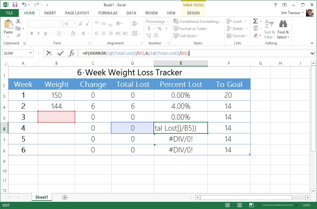
The way we combine the IF and ISERROR functions is by using ISERROR as the test for an IF statement. Let’s turn to our weight loss spreadsheet as an example. The reason that cell E6 is returning a #DIV/0! error is because its formula is attempting to divide the total weight lost by the previous week’s weight, which isn’t yet available for all weeks and which effectively acts as trying to divide by zero.
But if we use a combination of IF and ISERROR, we can tell Excel to ignore the errors and just enter 0% (or any value we want), or simply complete the calculation if no errors are present. In our example, this can be accomplished with the following formula:
IF(ISERROR(D6/B5),0,(D6/D5))
To reiterate, the formula above says that if the answer to D6/D5 results in an error [IF(ISERROR(D6/B5),0,(D6/D5))], then return a value of zero [IF(ISERROR(D6/B5),0,(D6/D5))]. But if D6/B5 does not result in an error, then simply display the solution to that calculation [IF(ISERROR(D6/B5),0,(D6/D5))].
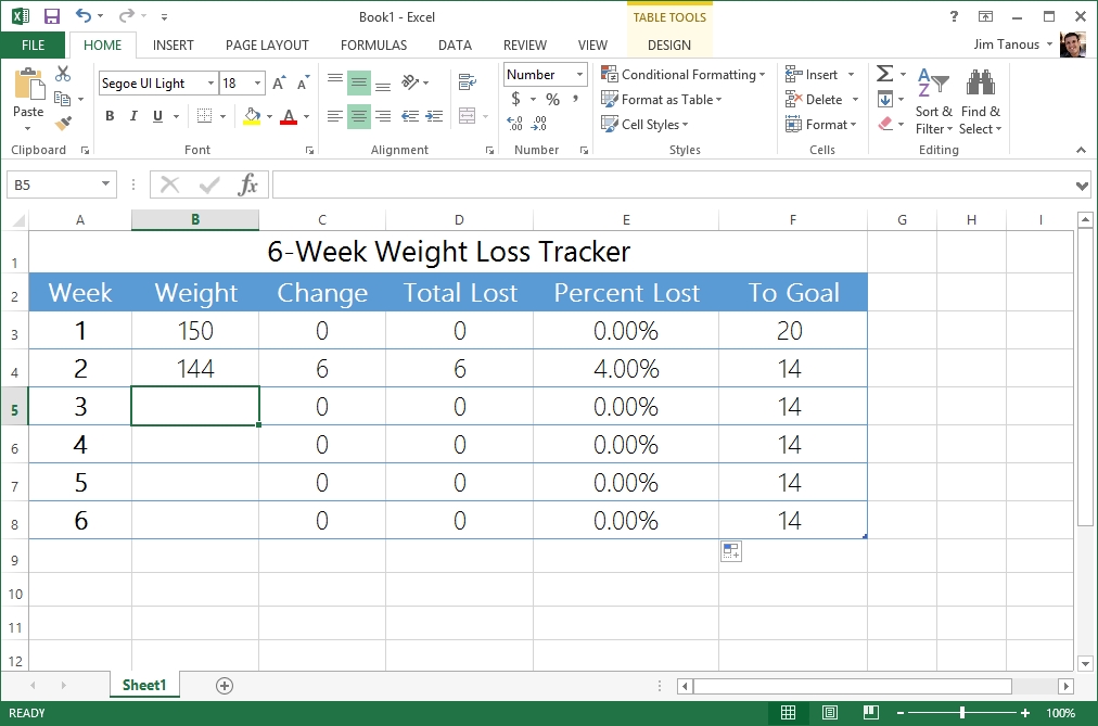
With that function in place, you can copy it to any remaining cells and any errors will be replaced with zeros. However, as you enter new data in the future, the affected cells will automatically update to their correct values because the error condition will no longer be true.

Keep in mind that when trying to hide Excel errors you can use just about any value or formula for all three variables in the IF statement; it doesn’t have to be a zero or whole number like in our example. Alternatives include referencing an entirely separate formula or inserting a blank space by using two quotation marks (“”) as your “true” value. To illustrate, the following formula would display a blank space in the event of an error instead of a zero:
IF(ISERROR(D6/B5),"",(D6/D5))
Just remember that IF statements can quickly become lengthy and complicated, especially when paired with ISERROR, and it’s easy to misplace a parentheses or comma in such situations. Recent versions of Excel color code formulas when you enter them to help you keep track of cell values and parentheses.


One thought on “How to Hide Excel Errors with the IF and ISERROR Functions”